Sight reduction with matrix algebra and least squares

Sight Reduction with Matrices — R. Watkins & P. M. Janiczek (1978)

1.  Description

The Watkins & Janiczek method is a technique for computing the astronomical fix from any number of lines of position, expressing the problem in the compact form of matrix algebra and solving it by the least-squares criterion. It was published by Robert Watkins and Paul M. Janiczek in 1978 in NAVIGATION, the journal of the Institute of Navigation, under the title “Sight Reduction with Matrices”.

The problem it addresses is as old as celestial navigation itself: when three or more bodies are observed, the resulting lines of position almost never pass through a single point. Instead they form a small error polygon — the famous “cocked hat” — and the navigator must decide which point to adopt as the most probable position. The traditional graphical solution is to plot the lines on the chart and estimate the centre of the triangle by eye. Watkins and Janiczek replace this with a rigorous, repeatable calculation that is easily programmed on a calculator or computer.

The key idea is elegant: each line of position is linearised about the dead-reckoning position (DR) and written as a linear equation in the two unknowns ΔLat and ΔLon. With n sights one obtains a system of n equations in 2 unknowns — over-determined — whose least-squares solution gives directly the offset from the DR and hence the observed position.

2.  The problem: a fix from n lines of position

To understand the method we must recall the intercept principle (Marcq St. Hilaire), on which all modern celestial navigation rests. From each observation of a body a line of position is derived as follows:

• The body’s altitude is measured with the sextant and, after corrections (index error, dip of the horizon, refraction, and where relevant parallax and semidiameter), the observed altitude Ho is obtained.
• For the dead-reckoning position (DR) and the instant of the observation, the computed altitude Hc and the azimuth Zn of the body are obtained from the ephemerides.

The difference a = Ho − Hc, called the intercept, expressed in arc minutes equals nautical miles: it measures how far our true position lies from the DR in the direction of the body. If a is positive the vessel is closer to the body (the intercept is laid off toward the azimuth); if negative, farther away.

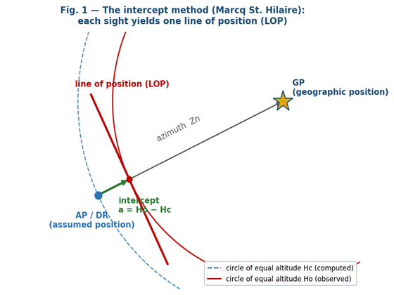
Figure 1 — Each sight yields one line of position, tangent to the circle of equal altitude and perpendicular to the azimuth.

A single sight gives one line: the vessel is somewhere along it. At least two bodies are needed for a fix; in practice three or more are observed to check for errors. But more lines inevitably bring the error triangle of Figure 2.

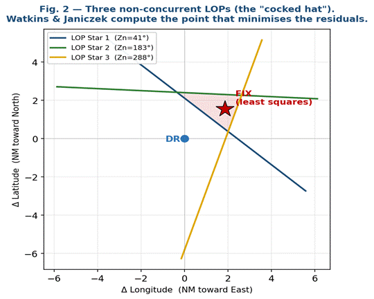
Figure 2 — Three lines of position affected by small errors do not concur in a point: the Watkins & Janiczek method finds the fix that minimises the sum of the squared residuals.

3.  How it works

The heart of the method is the linearisation of the line of position. Near the DR, the circle of equal altitude (which is in fact a circle of enormous radius on the Earth’s sphere) can be approximated by its tangent: a straight line. This line is perpendicular to the azimuth Zn and lies at the intercept distance a from the DR along the azimuth direction.

Let ΔLat be the northward displacement of the fix relative to the DR (in nautical miles) and ΔLon′ the eastward displacement, also in miles (the so-called departure). The condition “the point lies on the line of position of body i” translates into the linear equation:

cos Znᵢ · ΔLat  +  sin Znᵢ · ΔLon′  =  aᵢ

This relation, illustrated in Figure 3, is simply the projection of the intercept onto the two axes North and East: the intercept a, directed along the azimuth Zn, has northward component a·cos Zn and eastward component a·sin Zn.

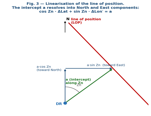
Figure 3 — Linearisation: the equation of each line of position arises from resolving the intercept along the North and East axes.

With n bodies we obtain n equations of this kind. Since there are only two unknowns (ΔLat and ΔLon′), for n ≥ 3 the system is over-determined: in general no point satisfies all equations exactly, because every observation carries small errors. Watkins and Janiczek therefore collect the n equations in matrix form and seek the solution that minimises the sum of the squared residuals.

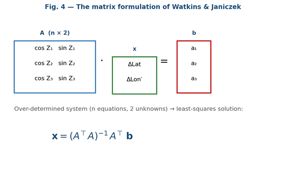
Figure 4 — The matrix form A·x = b and its least-squares solution, the core of the method.

4.  The formulae

4.1  Matrix form

Arranging the coefficients of the n equations in a matrix A (n rows, 2 columns), the unknowns in the vector x and the intercepts in the vector b:

A · x = b

where the rows of A are [cos Znᵢ , sin Znᵢ], x = [ΔLat ; ΔLon′] and b = [a₁ ; a₂ ; … ; aₙ]. The least-squares solution — the one that minimises |A·x − b|² — follows from the normal equations:

x = (Aᵀ A)⁻¹ Aᵀ b

4.2  Explicit form (the five sums)

Expanding the product AᵀA, which is a 2×2 matrix, the method reduces to computing five sums taken over all n observations. This is the practical, directly programmable form that Watkins and Janiczek emphasise:

A = Σ cos²Znᵢ      B = Σ cosZnᵢ·sinZnᵢ      C = Σ sin²Znᵢ

D = Σ aᵢ·cosZnᵢ      E = Σ aᵢ·sinZnᵢ

The system of normal equations then becomes the 2×2 system:

A·ΔLat + B·ΔLon′ = D

B·ΔLat + C·ΔLon′ = E

whose solution, with the determinant G = A·C − B², is:

ΔLat = (C·D − B·E) / G       ΔLon′ = (A·E − B·D) / G

4.3  From departure to longitude

ΔLat and ΔLon′ are both in nautical miles. ΔLat is added directly to the DR latitude (1′ of latitude = 1 NM). For longitude, the departure ΔLon′ must instead be divided by the cosine of the latitude, because the meridians converge toward the poles:

Lat_fix = Lat_DR + ΔLat⁄₆₀       Lon_fix = Lon_DR + ΔLon′ ⁄ (60·cos Lat)

4.4  Quality control: the residuals

Once the fix is found, for each body the residual is computed — the gap between the observed intercept and the one predicted by the fix:

rᵢ = aᵢ − (ΔLat·cos Znᵢ + ΔLon′·sin Znᵢ)

Small residuals (typically under half a mile) indicate consistent observations and a reliable fix; an anomalous residual instead flags a faulty observation, which can be discarded and the calculation repeated.

5.  Step-by-step procedure

1. For each body, reduce the sight by the intercept method: compute Hc and Zn from the DR and the time, derive Ho from the sextant corrections, and hence the intercept a = Ho − Hc.
2. For each body compute the products cos Zn, sin Zn and accumulate the five sums A, B, C, D, E.
3. Compute the determinant G = A·C − B².
4. Solve for ΔLat and ΔLon′ with the Cramer formulae of section 4.2.
5. Convert ΔLon′ to a difference of longitude by dividing by cos Lat, and apply ΔLat and ΔLon to the DR to obtain the fix.
6. Compute the residuals to verify the consistency of the observations; if necessary, discard the anomalous body and recompute.

6.  Worked example

Consider three bodies of a classic twilight fix: dead-reckoning position DR N 53°29′ E 008°00′, date 26 June 2014. Reducing the three sights gives the azimuths and intercepts shown in the table below.

Star	Zn (azimuth)	Intercept a	Sense
Schedar	40.83°	+1.58 NM	toward
Rasalhague	183.10°	−2.42 NM	away
Alkaid	288.40°	−1.84 NM	away

Accumulating the five Watkins & Janiczek sums over these three bodies gives:

Sum	Value (example)
A = Σ cos²Zn	1.66923
B = Σ cosZn·sinZn	0.24920
C = Σ sin²Zn	1.33077
D = Σ a·cosZn	3.03118
E = Σ a·sinZn	2.90983
G = A·C − B²  (determinant)	2.15926

Solving the 2×2 system:

ΔLat = (C·D − B·E)⁄G = +1.53 NM       ΔLon′ = (A·E − B·D)⁄G = +1.90 NM

Applying the offsets to the DR (with cos 53°29′ ≈ 0.595 for the longitude) gives the observed position:

FIX = N 53°30.5′   E 008°03.2′

2.44 miles from the DR, with residuals of 0.52 – 0.82 NM on the three bodies: a small cocked hat and therefore a good-quality fix. (These are exactly the values produced by the “Punto Astronomico” Excel workbook, which implements the same method.)

7.  Strengths and limitations

Strengths

• Objective and repeatable: it removes the by-eye estimate of the centre of the error triangle.
• General: it treats 2, 3 or n observations in the same way, including bodies of different kinds (stars, Sun, Moon, planets).
• Compact and programmable: it reduces to five sums and a 2×2 system, ideal for programmable calculators and spreadsheets.
• It provides the residuals, and hence an immediate check on the quality of the observations.

Limitations

• It is a linearised method: it assumes the DR is reasonably close to the true position (within a few tens of miles). If the DR is far off, it is better to iterate — recompute using the fix as a new DR — until the offset becomes negligible.
• Ordinary least squares weights all observations equally: undetected gross errors can distort the fix. Hence the importance of checking the residuals.
• It does not by itself correct for the vessel’s run between observations: the altitudes must be reduced to a common instant (“run up”) before the calculation if the sights are not simultaneous.

8.  References

Watkins R., Janiczek P. M., “Sight Reduction with Matrices”, NAVIGATION: Journal of the Institute of Navigation, Vol. 25, No. 4, 1978–79, pp. 447–448.

The Nautical Almanac — Sight Reduction Procedures; HMNAO / USNO, Compact Data for Navigation and Astronomy.

Bowditch N., The American Practical Navigator, Pub. No. 9, ch. 20 — Sight Reduction.